Suitability Function#
SuitabilityFunction is used to convert indicator to suitability values. LSAPy support two types of suitability function: discrete function and membership function.
[1]:
# import libraries
from lsapy import SuitabilityFunction
# alternatively, you can import the class from the function module
# from lsapy.function import SuitabilityFunction
Discrete Suitability Function#
dict with the indicator value as key and the associated suitability as value.[2]:
x = [1, 2, 3, 4, 5]  # discrete indicator values
rules = {1: 0, 2: 0, 3: 0.2, 4: 0.6, 5: 1}  # suitability values

func = SuitabilityFunction(name="discrete", params={"rules": rules})  # initialize the function
func(x)
[2]:
array([0. , 0. , 0.2, 0.6, 1. ], dtype=float32)
str type indicators values is also supported.
[3]:
x = ["1", "2", "3", "4", "5"]  # discrete indicator values
rules = {"1": 0, "2": 0, "3": 0.2, "4": 0.6, "5": 1}  # suitability values

func = SuitabilityFunction(name="discrete", params={"rules": rules})  # initialize the function
func(x)
[3]:
array([0. , 0. , 0.2, 0.6, 1. ], dtype=float32)
Membership Suitability Function#
Membership functions are a bit more complex and are used to convert continuous indicators to suitability using a fuzzy-logic approach. Several membership functions are available allowing flexibility in the shape of the curve desired. The list of all implemented membership functions can be found here.
The first step is thus to determine which function we should use and with which parameters. The fit_membership function can be used to find the best membership function. Let’s say we have indicator value ranging from 750 to 2000 and we know that suitability values of 0, 0.25, 0.5, 0.75, 1 correspond respectively to 1000, 1150, 1250, 1350, 1500. We can use this information to fit membership functions and determine which one it the best.
[4]:
from lsapy.functions.membership import fit_membership

fit_membership(x=[1000, 1150, 1250, 1350, 1500], y=[0, 0.25, 0.5, 0.75, 1])
/tmp/ipykernel_2302/986613430.py:3: UserWarning: No parameters to determine for `sigmoid`. Skipped.
  fit_membership(x=[1000, 1150, 1250, 1350, 1500], y=[0, 0.25, 0.5, 0.75, 1])
/tmp/ipykernel_2302/986613430.py:3: UserWarning: Fitting does not support `vetharaniam2024_eq8`. Skipped.
  fit_membership(x=[1000, 1150, 1250, 1350, 1500], y=[0, 0.25, 0.5, 0.75, 1])
/home/docs/checkouts/readthedocs.org/user_builds/lsapy/conda/v0.2.0/lib/python3.13/site-packages/lsapy/functions/membership.py:249: RuntimeWarning: overflow encountered in exp
  return 2 / (1 + np.exp(a * np.power(np.power(x, c) - np.power(b, c), 2)))
/home/docs/checkouts/readthedocs.org/user_builds/lsapy/conda/v0.2.0/lib/python3.13/site-packages/lsapy/functions/membership.py:305: OptimizeWarning: Covariance of the parameters could not be estimated
  popt, _ = curve_fit(f, x, y, p0=p0, maxfev=15000)
[4]:
(<function lsapy.functions.membership.vetharaniam2022_eq5(x, a, b)>,
 array([-8.75896892e-01,  1.24843934e+03]))
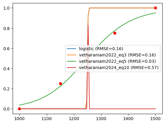
plot=True and verbose=True respectively.[5]:
fit_membership(x=[1000, 1150, 1250, 1350, 1500], y=[0, 0.25, 0.5, 0.75, 1], plot=True, verbose=True)
Best fit: vetharaniam2022_eq5
RMSE: 0.03187
Params: a=-0.8758968917667534, b=1248.43934103999
/tmp/ipykernel_2302/383407629.py:1: UserWarning: No parameters to determine for `sigmoid`. Skipped.
  fit_membership(x=[1000, 1150, 1250, 1350, 1500], y=[0, 0.25, 0.5, 0.75, 1], plot=True, verbose=True)
/tmp/ipykernel_2302/383407629.py:1: UserWarning: Fitting does not support `vetharaniam2024_eq8`. Skipped.
  fit_membership(x=[1000, 1150, 1250, 1350, 1500], y=[0, 0.25, 0.5, 0.75, 1], plot=True, verbose=True)
[5]:
(<function lsapy.functions.membership.vetharaniam2022_eq5(x, a, b)>,
 array([-8.75896892e-01,  1.24843934e+03]))
We can now use the results of the fitting to convert indicator value into suitability.
[6]:
import numpy as np

func = SuitabilityFunction(name="vetharaniam2022_eq5", params={"a": -0.876, "b": 1248})
x = np.linspace(750, 2000, 100)  # indicator values: create a array of 100 values between 750 and 2000
func(x)
[6]:
array([9.5176324e-04, 1.1635135e-03, 1.4199546e-03, 1.7300220e-03,
       2.1043362e-03, 2.5554982e-03, 3.0984317e-03, 3.7507790e-03,
       4.5333509e-03, 5.4706451e-03, 6.5914313e-03, 7.9294061e-03,
       9.5239300e-03, 1.1420826e-02, 1.3673263e-02, 1.6342668e-02,
       1.9499702e-02, 2.3225209e-02, 2.7611116e-02, 3.2761227e-02,
       3.8791765e-02, 4.5831595e-02, 5.4021928e-02, 6.3515328e-02,
       7.4473821e-02, 8.7065808e-02, 1.0146171e-01, 1.1782788e-01,
       1.3631900e-01, 1.5706876e-01, 1.8017919e-01, 2.0570910e-01,
       2.3366249e-01, 2.6397806e-01, 2.9652125e-01, 3.3107966e-01,
       3.6736408e-01, 4.0501490e-01, 4.4361451e-01, 4.8270488e-01,
       5.2180916e-01, 5.6045455e-01, 5.9819460e-01, 6.3462907e-01,
       6.6941839e-01, 7.0229357e-01, 7.3305970e-01, 7.6159453e-01,
       7.8784293e-01, 8.1180829e-01, 8.3354247e-01, 8.5313523e-01,
       8.7070388e-01, 8.8638395e-01, 9.0032142e-01, 9.1266620e-01,
       9.2356694e-01, 9.3316752e-01, 9.4160432e-01, 9.4900465e-01,
       9.5548576e-01, 9.6115464e-01, 9.6610790e-01, 9.7043228e-01,
       9.7420520e-01, 9.7749531e-01, 9.8036349e-01, 9.8286319e-01,
       9.8504144e-01, 9.8693955e-01, 9.8859352e-01, 9.9003494e-01,
       9.9129134e-01, 9.9238664e-01, 9.9334168e-01, 9.9417472e-01,
       9.9490154e-01, 9.9553591e-01, 9.9608976e-01, 9.9657345e-01,
       9.9699605e-01, 9.9736547e-01, 9.9768847e-01, 9.9797100e-01,
       9.9821824e-01, 9.9843472e-01, 9.9862427e-01, 9.9879038e-01,
       9.9893600e-01, 9.9906373e-01, 9.9917573e-01, 9.9927408e-01,
       9.9936038e-01, 9.9943620e-01, 9.9950284e-01, 9.9956143e-01,
       9.9961299e-01, 9.9965835e-01, 9.9969822e-01, 9.9973339e-01],
      dtype=float32)
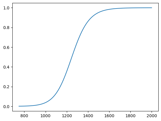
[7]:
func.plot(x)