Suitability Criteria#

NOTE: If you are not familiar with the different suitability functions and how to use them, we recommend you start with the Suitability Functions tutorial, which provides an overview of the available functions and their usage.

SuitabilityCriteria is used to defined a criteria, set its associated indicator, and described how its suitability is computed. It has the following attributes:

name: criteria name
indicator: input data to compute suitability
func (SuitabilityFunction): suitability function to use
weight (default=1): criteria weight used when computing land suitability
category (optional): criteria category allowing to compute land suitability for different category (e.g., climate, soil…)
long_name: criteria long name
description: description of the criteria
comment: additional information
is_computed (bool, default=False): specify if the indicator data already corresponds to it’s suitability.

Below is an example using LSAPy open_data utility function to download and open sample data:

[1]:

from lsapy import SuitabilityCriteria, SuitabilityFunction
from lsapy.utils import open_data

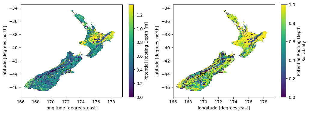
potential_rooting_depth = open_data("land", variables="potential_rooting_depth")

sc = SuitabilityCriteria(
    name="potential_root_depth",
    long_name="Potential Rooting Depth Suitability",
    indicator=potential_rooting_depth,
    func=SuitabilityFunction(name="vetharaniam2022_eq5", params={"a": -11.98, "b": 0.459}),
)

Downloading file 'nzglid_5km.zip' from 'doi:10.5281/zenodo.16249350/nzglid_5km.zip' to '/home/docs/.cache/lsapy'.
Extracting 'NZGLID_potential-rooting-depth_NZ5km.nc' from '/home/docs/.cache/lsapy/nzglid_5km.zip' to '/home/docs/.cache/lsapy/nzglid_5km.zip.unzip'

We can now compute the suitability of the criteria and plot the result.

[2]:

import matplotlib.pyplot as plt

prd = sc.compute()

fig, ax = plt.subplots(1, 2, figsize=(12, 4))
potential_rooting_depth.plot(ax=ax[0])
prd.plot(ax=ax[1], vmin=0, vmax=1)
plt.show()

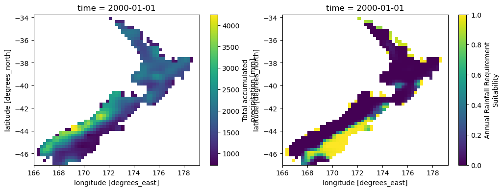
Let’s see another example with climate data. We use xclim package to calculate the total annual precipition and use this latter as criteria indicator.

[3]:

from xclim.indicators.atmos import precip_accumulation

precip = open_data("climate", variables="pr")

prtot = precip_accumulation(precip, freq="YS")  # YS: Year Start frequency

sc = SuitabilityCriteria(
    name="water_requirements",
    long_name="Annual Rainfall Requirement Suitability",
    indicator=prtot,
    func=SuitabilityFunction(name="vetharaniam2022_eq5", params={"a": 0.876, "b": 1248}),
)

Downloading file 'NEX-GDDP-CMIP6_day_ACCESS-CM2_historical_r1i1p1f1_20000101-20041231.nc' from 'https://raw.githubusercontent.com/baptistehamon/lsapy/main/src/lsapy/data/NEX-GDDP-CMIP6_day_ACCESS-CM2_historical_r1i1p1f1_20000101-20041231.nc' to '/home/docs/.cache/lsapy'.

[4]:

water_req = sc.compute()

fig, ax = plt.subplots(1, 2, figsize=(12, 4))
prtot.isel(time=0).plot(ax=ax[0])  # use first year of data as example
water_req.isel(time=0).plot(ax=ax[1], vmin=0, vmax=1)
plt.show()