Land Suitability Analysis#

NOTE: If you are new to LSAPy, we recommend you start with the Suitability Criteria tutorial.

To perform a LSA, we use LandSuitabilityAnalysis that allows to compute the overall suitability of several criteria and that has the following attributes:

land_use: a name for the land use.
criteria: dict of SuitabilityCriteria where the keys is the name of the criteria.
short_name (optional): a short name for the land suitability analysis (LSA).
long_name (optional): a long name for the LSA.
description (optional): additional information about the LSA.
comment (optional): miscellaneous information about the LSA.

First we have to define the criteria. Here, we use three criteria: the potential rooting depth, the soil draingage class (discrete) and water requirement. We are going to split criteria in two categories, soil and climate, and change the weight of each of them.

[1]:

import matplotlib.pyplot as plt
from xclim.indicators.atmos import precip_accumulation

import lsapy.standardize as lstd
from lsapy import LandSuitabilityAnalysis, SuitabilityCriteria
from lsapy.utils import open_data

soil_data = open_data("land", variables=["potential_rooting_depth", "drainage"])
pr = open_data("climate", variables="pr").interp_like(
    soil_data,
    method="nearest",  # resample precipitation data to soil data resolution
)

Extracting 'NZGLID_potential-rooting-depth_5km_v2.0.nc' from '/home/docs/.cache/lsapy/nzglid_5km_v2.0.zip' to '/home/docs/.cache/lsapy/nzglid_5km_v2.0.zip.unzip'
Extracting 'NZGLID_drainage_5km_v2.0.nc' from '/home/docs/.cache/lsapy/nzglid_5km_v2.0.zip' to '/home/docs/.cache/lsapy/nzglid_5km_v2.0.zip.unzip'

[2]:

lsa = LandSuitabilityAnalysis(
    land_use="your_land_use",
    long_name="My First Land Suitability Analysis",
    criteria={
        "potential_root_depth": SuitabilityCriteria(
            name="potential_root_depth",
            long_name="Potential Rooting Depth Suitability",
            weight=2,
            category="soil",
            indicator=soil_data["potential_rooting_depth"],
            func=lstd.vetharaniam2022_eq5,
            fparams={"a": -11.98, "b": 0.459},
        ),
        "drainage_class": SuitabilityCriteria(
            name="drainage_class",
            weight=1,
            category="soil",
            long_name="Drainage Class Suitability",
            indicator=soil_data["drainage"],
            func=lstd.discrete,
            fparams={"rules": {0: 0, 1: 0.1, 2: 0.5, 3: 0.9, 4: 1}},
        ),
        "water_requirements": SuitabilityCriteria(
            name="water_requirements",
            weight=0.5,
            category="climate",
            long_name="Annual Rainfall Requirement Suitability",
            indicator=precip_accumulation(pr, freq="YS"),
            func=lstd.vetharaniam2022_eq5,
            fparams={"a": 0.876, "b": 1248},
        ),
    },
)

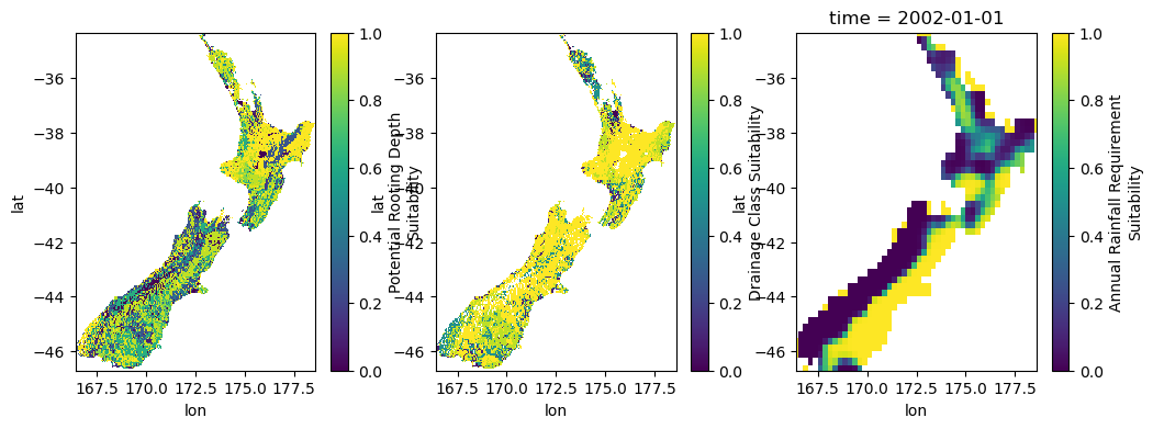
Then, we can compute the suitability starting with the criteria.

[3]:

lsa.run(suitability_type="criteria", inplace=True)
lsa.data

[4]:

fig, ax = plt.subplots(1, 3, figsize=(12, 4))
lsa.data["potential_root_depth"].plot(ax=ax[0], vmin=0, vmax=1)
lsa.data["drainage_class"].plot(ax=ax[1], vmin=0, vmax=1)
lsa.data["water_requirements"].isel(time=2).plot(ax=ax[2], vmin=0, vmax=1)
plt.show()

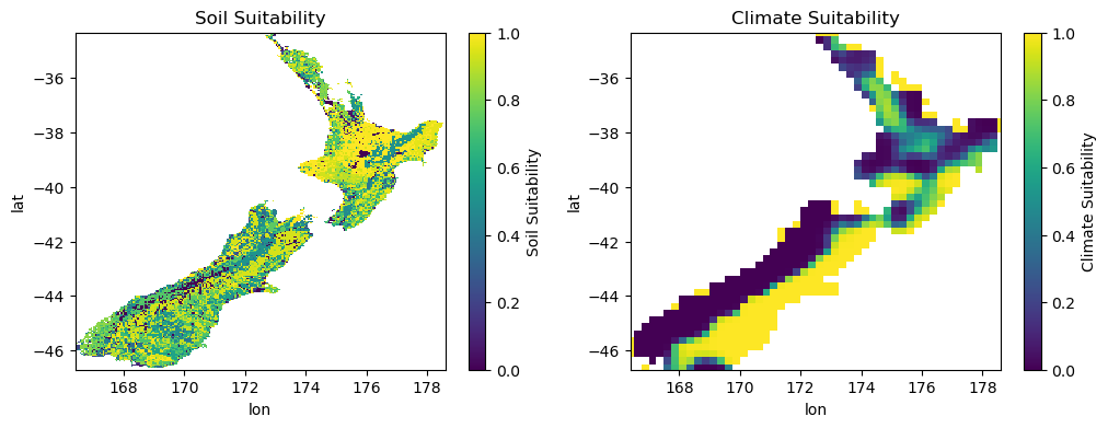
Now, we can compute the suitability of categories. There are several method implemented to aggregate criteria (e.g., mean, weighted mean, geometric mean, weighted geometric mean, and limiting factor). Here, we are going to use a simple weighted mean.

[5]:

lsa.run(suitability_type="category", agg_methods="wmean", keep_vars=True, inplace=True)
lsa.data

/tmp/ipykernel_2316/1253614186.py:1: UserWarning: Existing data found and will be overwritten.
  lsa.run(suitability_type="category", agg_methods="wmean", keep_vars=True, inplace=True)

[6]:

fig, ax = plt.subplots(1, 2, figsize=(12, 4))
lsa.data["soil"].plot(ax=ax[0], vmin=0, vmax=1)
ax[0].set_title("Soil Suitability")
lsa.data["climate"].isel(time=2).plot(ax=ax[1], vmin=0, vmax=1)
ax[1].set_title("Climate Suitability")
plt.show()

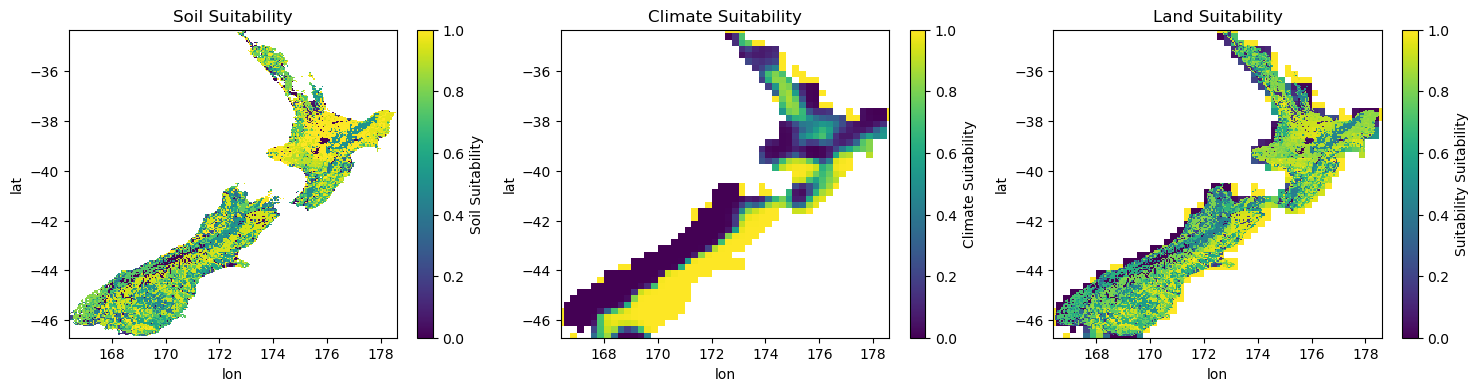
Finally, we can compute the overall suitability.

[7]:

lsa.run(suitability_type="overall", agg_methods="wmean", by_category=True, inplace=True)
lsa.data

/tmp/ipykernel_2316/831129037.py:1: UserWarning: Existing data found and will be overwritten.
  lsa.run(suitability_type="overall", agg_methods="wmean", by_category=True, inplace=True)

[8]:

fig, ax = plt.subplots(1, 3, figsize=(18, 4))
lsa.data["soil"].plot(ax=ax[0], vmin=0, vmax=1)
ax[0].set_title("Soil Suitability")
lsa.data["climate"].isel(time=2).plot(ax=ax[1], vmin=0, vmax=1)
ax[1].set_title("Climate Suitability")
lsa.data["suitability"].isel(time=2).plot(ax=ax[2], vmin=0, vmax=1)
ax[2].set_title("Land Suitability")
plt.show()