Suitability Criteria#

SuitabilityCriteria is used to defined a criteria, set its associated indicator, and described how its suitability is computed. It has the following attributes:

name: criteria name
indicator: input data to compute suitability
func: standardization function used to compute land suitability
fparams: function parameters
weight (default=1): criteria weight used when computing land suitability
category (optional): criteria category allowing to compute land suitability for different category (e.g., climate, soil…)
long_name: criteria long name
description: description of the criteria
comment: additional information
is_computed (bool, default=False): specify if the indicator data already corresponds to it’s suitability.

Below is an example using LSAPy open_data utility function to download and open sample data:

[1]:

import lsapy.standardize as lstd
from lsapy import SuitabilityCriteria
from lsapy.utils import open_data

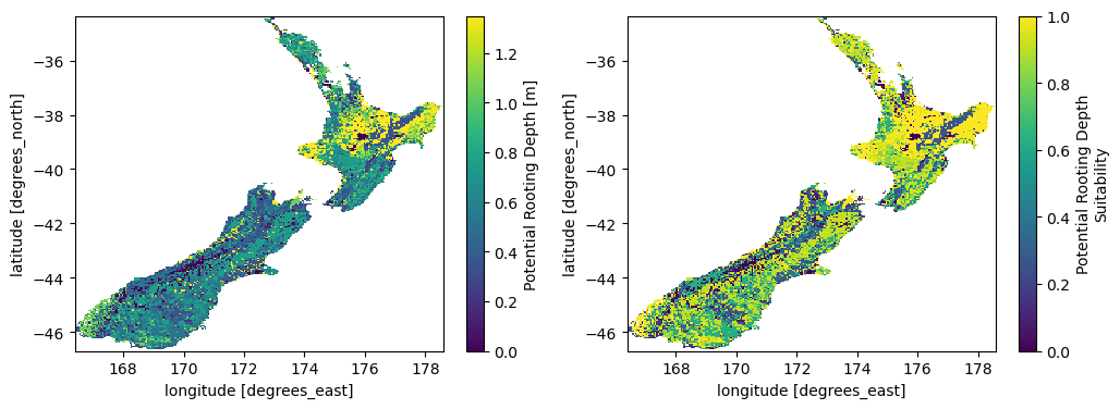
potential_rooting_depth = open_data("land", variables="potential_rooting_depth")

sc = SuitabilityCriteria(
    name="potential_root_depth",
    long_name="Potential Rooting Depth Suitability",
    indicator=potential_rooting_depth,
    func=lstd.vetharaniam2022_eq5,
    fparams={"a": -11.98, "b": 0.459},
)

Downloading file 'nzglid_5km_v2.0.zip' from 'doi:10.5281/zenodo.19901807/nzglid_5km_v2.0.zip' to '/home/docs/.cache/lsapy'.
Extracting 'NZGLID_potential-rooting-depth_5km_v2.0.nc' from '/home/docs/.cache/lsapy/nzglid_5km_v2.0.zip' to '/home/docs/.cache/lsapy/nzglid_5km_v2.0.zip.unzip'

We can now compute the suitability of the criteria and plot the result.

[2]:

import matplotlib.pyplot as plt

prd = sc.compute()

fig, ax = plt.subplots(1, 2, figsize=(12, 4))
potential_rooting_depth.plot(ax=ax[0])
prd.plot(ax=ax[1], vmin=0, vmax=1)
plt.show()

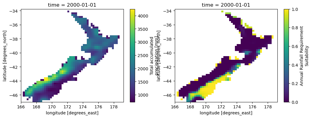
Let’s see another example with climate data. We use xclim package to calculate the total annual precipition and use this latter as criteria indicator.

[3]:

from xclim.indicators.atmos import precip_accumulation

precip = open_data("climate", variables="pr")

prtot = precip_accumulation(precip, freq="YS")  # YS: Year Start frequency

sc = SuitabilityCriteria(
    name="water_requirements",
    long_name="Annual Rainfall Requirement Suitability",
    indicator=prtot,
    func=lstd.vetharaniam2022_eq5,
    fparams={"a": 0.876, "b": 1248},
)

Downloading file 'NEX-GDDP-CMIP6_day_ACCESS-CM2_historical_r1i1p1f1_20000101-20041231.nc' from 'https://raw.githubusercontent.com/baptistehamon/lsapy/main/src/lsapy/data/NEX-GDDP-CMIP6_day_ACCESS-CM2_historical_r1i1p1f1_20000101-20041231.nc' to '/home/docs/.cache/lsapy'.

[4]:

water_req = sc.compute()

fig, ax = plt.subplots(1, 2, figsize=(12, 4))
prtot.isel(time=0).plot(ax=ax[0])  # use first year of data as example
water_req.isel(time=0).plot(ax=ax[1], vmin=0, vmax=1)
plt.show()